By Malcolm P.R. Light
August 10, 2012
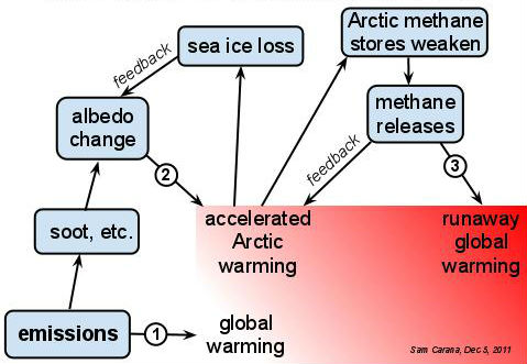
Abstract The exponential increase in the Arctic atmospheric methane derived from the destabilization of the subsea Arctic methane hydrates is defined by both the exponential decrease in the volume of Arctic sea ice due to global warming and the exponential decrease in the continent wide reflectivity (albedo) of the Greenland ice cap caused by increasing rates of surface melting which reach minima around 2014, 2015.
The high anomalous atmospheric methane contents recorded this year at Barrow Point Alaska (up to 2500 ppb - Carana 2012b) and the fact that the surface atmospheric methane contents may be linked via a stable partial pressure gradient with increased maximum methane contents in the world encompassing global warming veil (estimated at ca 1460 ppb methane) makes it imperative that the Merlin lidar satellite be launched as soon as is feasibly possible. The Merlin lidar satellite will give us a clear idea of how high the Earth’s stratospheric methane concentrations are in this poorly documented giant methane reservoir formed above the ozone layer at 30 km to 50 km altitude (Ehret, 2010).
Methane detecting Lidar instruments could also be installed immediately on the International Space Station to give early warning of the methane buildup in the stratosphere and act as a back up in case the Merlin satellite fails.
Unless immediate and concerted action is taken by governments and oil companies to depressurize the Arctic subsea methane reserves by extracting the methane, liquefying it and selling it as a green house gas energy source, rising sea levels will breach the Thames Barrier by 2029 flooding London. The base of the Washington Monument (D.C.) will be inundated by 2031. Total global deglaciation will finally cause the sea level to rise up the lower 35% of the Washington Monument by 2051 (68.3 m or 224 feet above present sea level).
IntroductionRecent atmospheric methane observations (May 01, 2012) at Barrow Point Alaska show extreme methane concentrations as high as 2500 ppb (2.5 ppm Methane, Figure 1)(Generated by ESRL/GMD May 01, 2012 from Carana, 2012b). The present atmospheric methane concentration at Point Barrow exceeds all previous measurements in the Arctic and if it represented the mean atmospheric concentration after an extended period of subsea Arctic methane emission (10 to 20 years) at a methane global warming potential (GWP) of 100 (Dessus et al. 2008) it would be equal to a 2.5 degrees C mean global temperature increase and a methane-carbon output of some 6 Gt. This would be equivalent to adding and extra 250 ppm of carbon dioxide to the atmosphere or about 2/3 of the present carbon dioxide content.

The rising light Arctic methane migration routes have been interpreted on the Hippo profile in Figure 2a (from Wofsy et al. et al. 2009) using the inflexion points on the temperature and methane concentration profiles similar to the system used to identify deep oceanic current trends using salinity and temperature data (Tharp and Frankel, 1986). The light Arctic methane is rising almost vertically up to the stratosphere between 60o North and the North Pole. This is consistent with the methane rising in the same way as hydrogen with respect to the cold dry polar air because it has almost half the density of air at STP(Engineering Toolbox, 2011) (methane in wet air may be transported horizontally by storm systems). In addition because methane has a global warming potential of close to 100 during the first 15 to 20 years of its life (Dessus et al. 2001) it will preferentially warm up and expand compared to the other atmospheric gases and thus drop even further in density making it much lighter than the air. This methane rises into the upper stratosphere where it is trapped below the hydrogen against which it has an upper diffuse boundary as shown by the fall off in methane concentration between 40 km and 50 km altitude (Figure 2a after Nassar et al. 2005).
It is clear from the flattening of the methane concentration trend in the stratosphere between 30 km and 47 km (Nassar et al. 2005) that this probably represents an expanding, world encompassing methane global warming veil (Figure 2a after Nassar et al. 2005). This stratospheric methane is above the ozone layer and it appears entirely stable between 30 km and 40 km where it shows little change (Figure 2a after Nassar et al. 2005). It is therefore very likely that the methane global warming veil will form a giant reservoir for quickly rising low density methane emitted into the dry Arctic atmosphere by progressive destabilization of subsea Arctic methane hydrates (Light, 2011, 2012) combined with smaller amounts of methane formed by methanogenesis (Allen and Allen, 1990; Lopatin 1971). Much of the dry, light methane is able to bypass the ozone layer unimpeded in a tropospheric - stratospheric circulation system to be discussed later.
There is a transition zone from about 60
o to 65
o North where the methane begins to spiral outwards from the Arctic region towards the mid latitudes and upwards towards the stratosphere to reach the base of the ozone layer where it is being mixed into the stratosphere by giant vortices active at different times (Light 2012; NSIDC 2011a).
The continuous vertical motion of the methane in the Arctic region as it rises to the stratosphere between 60
o to 65
o North which has a lateral motion impressed on it at lower latitudes must set up a methane partial pressure - concentration gradient between the Arctic surface atmospheric methane emissions and the stratospheric methane global warming veil. Therefore any marked increase in the surface methane concentration and partial pressure should be marked by similar increases in the upper stratosphere within the methane global warming veil.
A further consequence of the light methane rising like hydrogen into the upper stratosphere where it forms a stable zone beneath the hydrogen between 30 km and 50 km height, is that this methane is never recorded in the mean global warming gas measurements made at Mauna Loa. We therefore have a completely separate high reservoir for methane, which at the moment we only have vague information on and it may contain sufficient methane gas to multiply the Mauna Loa readings by a considerable amount.
Graphic Display of The Effects of the Methane Warming VeilFigure 2b is a graphic display of the atmosphere from 0 to 55 km altitude versus increasing Arctic atmospheric methane concentration reaching up to 6000 ppb (6 ppmv methane). The troposphere, tropopause, stratosphere, stratopause, mesosphere, and ozone layer are from Heicklen, 1976. The various events related to global warming (droughts, water stress, coral bleaching and death, deglaciation, sea level rise and major global extinction) are from Parry et al. 2007.
Figure 2b has been designed to graphically portray the growth of the subsea Arctic atmospheric methane as new observations become available and how this build up strengthens the methane concentration in the stratosphere where it forms a world encompassing methane global warming veil at an altitude of 30 km to 47 km. Figure 2b will be used to progressively chart mankind's Arctic methane emission, exponential expressway to extinction within the next half century.
As the light-rising Arctic methane is spread around the world by the Arctic stratospheric vortex system (NSIDC 2011a), it can be expected to lead to more ozone and water vapor in the stratosphere, both of which will add to the greenhouse effect and thus cause temperatures to increase globally. In the Arctic, where there is very little water vapour in the atmosphere, the ozone layer may well be further depleted, because the rising methane behaves like a chloro-fluoro-hydrocarbon (CFC) under the action of sunlight increasing the damaging effects of ultraviolet radiation on the Earth’s surface (Engineering Toolbox, 2011; Anitei, 2007). Large abrupt releases of methane in the Arctic lead to high local concentrations of methane in the atmosphere and hydroxyl depletion, making that methane will persist longer at its highest warming potential, i.e. of over 100 times that of carbon dioxide. (Carana, 2011a). The presence of a large hole in the Arctic ozone layer in 2011 is most likely a result of this same process of ozone depletion caused by a buildup of greenhouse gases from the massive upward transfer of methane from the Arctic emission zones through the lower stratosphere up into the stratospheric veil between 30 km and 47 km height (Science Daily, 2011).
Anomalous Arctic Atmospheric Methane ConcentrationsThe extremely high content of atmospheric methane measured in May 2012 at Barrow Point Alaska (2500 ppb) represents a very dangerous turn of events in the Arctic and further substantiates the claim that the whole Arctic has now become a latent subsea methane hydrate sourced blowout zone which will require immediate remedial action if there is any faint hope of containing the now fast increasing (exponential!) rates of methane eruptions into the atmosphere (Light 2012c - Angels proposal; see end of this text).
The exponential increase in the Arctic atmospheric methane content from the destabilization of the subsea methane hydrates is defined by the exponential decrease in the volume of Arctic sea ice caused by the resulting global warming due to the build up of the atmospheric methane (Carana, 2012d). The exponential increase in the Arctic atmospheric methane is also implied by an exponential decrease in the continent wide reflectivity (albedo) of the Greenland ice cap caused by increasing rates of surface melting (Figure 3; NASA Mod 10A1 data, from Carana, 2012c).

Albedo data for Greenland shows that it will become free of a continuous snow cover by about 2014, so that the underlying old ice cover which has low reflectivity will be totally exposed to the sun in the summer (Carana, 2012c). This darker material will become a major heat absorber after 2014 starting the fast melt down of the Greenland ice cap and this process will probably affect the older ice in the floating Arctic sea ice fields. The Arctic ocean will also become free of sea ice by 2015 exposing the low reflectivity ocean water directly to the sun, causing a high rate of temperature rise in Arctic waters and the consequent destabilization of shelf and slope methane hydrates releasing large volumes of methane into the atmosphere (Carana, 2012d; AIRS data Yurganov, 2012).
As a consequence, the enhanced global warming will melt the global ice sheets at a fast increasing rate causing the sea level to begin rising at 15.182 cm/yr in the first few years after 2015 giving an accurate way of gauging the worldwide continental ice loss (Figure 3). This sudden increase in the rate of sea level rise will mark the last moment mankind will have to take control of the Arctic wide blowout of methane into the atmosphere and a massive effort must be made by governments and oil companies to stem the flow of the erupting subsea methane in the Arctic before this time. The loss of complete snow cover in Greenland precedes the loss of the sea ice cap in the Arctic by a year which may be due to the more extreme weather conditions that usually prevail over continents than over the sea which moderates the weather.
Methane and Ozone CirculationThe components of the atmosphere undergo diffusion by a number of processes. The mean speed of horizontal displacement of the stratosphere around the Earth is known to be about 120 km/hr from the Krakatoa eruption in 1883 (Heicklen, 1976). Winds also transfer material northward and southward in the stratosphere in quite a different pattern to that of the tropospheric wind flows (Heicklen, 1976). Mean wind velocities within the global methane warming veil and above it (36 km to 91 km altitude) are some 48 m/sec during the day and 56 m/sec at night (Olivier 1942, 1948). Large latitudinal variations in the atmospheric density at 100 km altitude require meridional flows of 10 to 50 m/sec (Heicklen, 1976).
At subarctic latitudes at the height of the global methane warming veil (30 km to 50 km altitude) the ozone concentration lies between 1.7 to 1.9*10^12 molecules/cc to 5.4*10^10 molecules/cc and does not vary during the day (Heicklen, 1976). The sub-arctic ozone reaches a maximum in the lower stratosphere in winter at an altitude of 17 km to 19 km (7.7*10^12 molecules/cc) and in summer at an altitude of 18 km to 19 km (5.1*10^12 molecules/cc)(Heicklen, 1976).
The seasonal variation of ozone in the stratosphere in Arctic latitudes is caused by a circulation transfer system which moves ozone from the upper stratosphere in equatorial and mid-latitudes to the Arctic lower stratosphere during the winter (Heicklen, 1976). The stored Arctic lower stratospheric ozone is lost in the summer by chemical dissociation when it moves downwards or by photosynthetic destruction if it moves upwards (Heicklen, 1976).
The Hippo methane concentration and temperature profiles shown in Figures 2a and 2b extend from the surface to some 14.4 km altitude and from the North Pole southwards across the Equator to a latitude of -40o south (Wofsy et al. 2009). As already described the methane flow trends on Hippo methane concentration and temperature profiles have been interpreted in detail using a similar system to that used by the Meteor expedition in determining deep ocean circulation patterns from salinity and temperature data (Figure 2a - see Tharp and Frankel, 1986).
Methane erupted from destabilizing methane hydrates in the subsea Arctic and of methanogenic origin has almost half the density of air at STP in dry Arctic conditions and is seen to be rising vertically to the top of the Troposphere between 70o North and the North Pole on the Hippo methane concentration profiles (Engineering Toolbox, 2011; Wofsy et al. 2009 ). On the Hippo data, at latitudes less than 70o North, the rising methane clouds are being spun out and laterally spread in the middle and upper troposphere and upper stratosphere by stratospheric vortices (NSIDC, 2011a). The methane appears to be entering the lower stratosphere in the low latitudes between 25o North and the equator which it then overlaps and is carried into the Southern Hemisphere to almost -40o South (Figure 2a)(Light 2011c). In the equatorial regions the growth of the methane global warming veil will amplify the effects of El Nino in the Pacific further enhancing its deleterious effects on the climate.
As this vertically and laterally migrating methane enters the stratosphere in equatorial and mid-latitude positions it is helping to displace the equatorial and mid-latitude ozone which migrates downwards and northwards towards the north pole (Heicklen, 1976) to complete the cycle. The methane may be partly drawn up into the lower and upper stratosphere by a global pressure differential set up by the poleward and downward motion of the ozone (Heicklen, 1976) Once the methane has entered the stratosphere and has helped to displace some of the ozone, it is able to accumulate in the upper stratosphere beneath the hydrogen as a continuous stable layer between 30 and 47 km forming a world wide global warming veil (Figures 2a and 2b; Light 2011c).
In the Arctic region methane has been shown to rise nearly vertically and is locally charging the global warming veil in addition to methane that has diffused from mid latitude and equatorial regions. There must therefore exist a partial pressure gradient between the Arctic surface methane anomalies and the upper stratosphere methane global warming veil such that any increase of the surface methane concentration and partial pressure should lead to a transfer of methane into the upper stratosphere and to a similar increase in the partial pressure and concentration of the methane there. The methane partial pressure gradient that exists between the anomalous Arctic ocean surface methane emissions and the stratospheric methane global warming veil at 30 km to 47 km height is partly controlled by the complex motions and reactions of the Arctic ozone layer which separates the troposphere from the upper stratosphere and shows little variation in the day or between summer and winter (Heicklen, 1976).
Consequently the concentration of the methane in the upper stratospheric global warming veil should track the increase of Arctic atmospheric methane to some degree and knowledge of the latter can allow absolute maximum estimates to be made on the magnitude of the former. This will give a rough estimate of what the highest value the methane concentration is likely to reach within the global warming veil within the Arctic area. This is a worst case scenario which has to be assumed in order to prevent Murphy’s law being operative (i.e. if anything can go wrong, it will go wrong in estimating the maximum methane value). An alternative is to view this solution of the methane concentration in the global warming veil as German over-engineering in order to eliminate any possible errors in the estimate of the maximum value. My Father, a Saxon would have commended me on this approach. This is precisely what mainstream world climatologists have failed to do in their modeling of the effects of Arctic methane hydrate emissions on the mean heat balance of the atmosphere and why we are now facing such a severe climatic catastrophe from which we may very likely not escape. Let us hope and pray that the Merlin Lidar methane detection satellite does not find methane magnitudes in the Arctic global warming methane veil (30 km – 47 km altitude) at the levels predicted in this paper, when it is launched in 2014.
The maximum global methane veil concentration in the mid latitudes (30
o to 60
o North) between 30 km and 40 km altitude was estimated by occultation at some 0.97 ppmv methane (970 ppb) between February to April, 2004 (Nassar et al. 2005). In 2004 - 2005 the Arctic atmosphere at Point Barrow, Alaska reached an anomalous maximum of some 2.014 ppmv methane (2014 ppb)(Carana, 2012e). This means that the most extreme methane concentration anomalies in the Arctic (Point Barrow) are leading the maximum concentration in the global warming methane veil by some 1.044 ppmv methane (1044 ppb). Consequently as a first rule of thumb assuming that the vertical methane partial pressure gradient has remained relatively unchanged, we can estimate the maximum methane concentration within the Arctic methane global warming veil between 30 km and 47 km height by subtracting 1.044 ppmv methane (1044 ppb) from measured surface Arctic atmospheric value at the same time.
High methane concentrations of 2 ppmv (2000 ppb) were being reached in the Arctic in 2011 (position a. in Figure 2b) similar to those recorded in 2004 – 2005 at Point Barrow Alaska (Carana, 2012e). It is therefore likely that by 2011 that the maximum concentration of methane in the methane global warming veil had remained relatively unchanged since 2004. This is consistent with the start of major methane emissions in the Arctic in August 2010 as recorded at the Svalbard station and in the East Siberian Shelf in 2011 which would not have given the emitted gases sufficient time to reach the upper stratosphere(Light, 2012a, Shakova et al. 2010a, b and c).
On May 01, 2012 an atmospheric methane concentration of 2.5 ppmv (2500 ppb) was recorded at Point Barrow indicating an increase in the maximum methane concentration anomaly of 0.5 ppmv methane (500 ppb) in one year (yellow spike on Figure 1; position b. in Figure 2b)(ESRL/GMO graph from Carana 2012b). We can therefore predict conservatively that the maximum concentration of the methane in the Arctic stratospheric methane global warming veil between 30 km and 47 km altitude may be as high as 1.456 ppmv methane (1456 ppb) (= 2500 -1044 ppmv) (position b. in Figure 2b)(ESRL/GMO graph from Carana 2012b).
Assuming that the maximum Arctic surface atmospheric methane content continues to increase now at a rate of 0.5 ppmv (500 ppb) each year we can roughly predict that by 2013 it will have reached 3 ppmv (3000 ppb) and by 2014, 3.5 ppmv (3500 ppb) which is when the Merlin Lidar methane detection satellite will be launched (Ehret, 2010). Using the previous method of predicting the maximum likely methane content in the Arctic methane global warming veil between 30 km and 47 km altitude, the maximum for 2013 is 1.956 ppmv methane (1956 ppb)(position c. in Figure 2b) and for 2014 is 2.456 ppmv methane (2456 ppb) (position d. in Figure 2b). This means that by the time the Merlin Lidar satellite is launched the Arctic Ocean will have emited sufficient methane to have surpassed the 2oC anomaly limit. Once the entire atmospheric mean exceeds a 2oC temperature increase it will precipitate fast deglaciation, the start of widespread inundation of worldwide coastlines, extensive droughts and water stress for billions of people (Figure 2b)(after Parry et al. 2007).
This high predicted concentration of methane in the Arctic methane global warming veil in 2014 is consistent with the exponentially falling albedo data for the Greenland ice cap which suggests that major melting will begin in 2014 (Carana, 2012c). The exponential reduction in volume of the Arctic sea ice to zero in 2015 (Carana, 2012d) will precipitate a massive increase in the release of Arctic subsea methane from destabilization of the methane hydrates as the dark ice free Arctic ocean absorbs large quantities of heat from the sun (Light, 2012a).
MERLIN Lidar SatelliteThe MERLIN lidar satellite (Methane Remote Sensing Lidar Mission) , which is a joint collaboration between France and Germany will orbit the Earth at 650 km altitude and will be able to detect the methane concentration in the atmosphere from 50 km altitude to the surface of the Earth (Ehret, 2010). The Lidar methane detection instrument was jointly developed by DLR (Deutches Zentrum für Luft –und Raumfahrt), ADLARES GmBH and E. ON Ruhrgas AG (Ehret, 2010).
This satellite is scheduled to be launched sometime in 2014 (Ehret, 2010) and will be the first time that real time data will be able to detect the concentration of methane within the world encompassing methane global warming veil between 30 km and 47 km altitude and give us the first detailed picture of the size of the beast we are dealing with. Previous indications of this layer in the mid latitudes was made using occultation (Nassar et al. 2005)
The high anomalous atmospheric methane contents recorded this year (May 01) at Barrow Point Alaska (see Figure 2b, Carana 2012b) and the fact that they may be linked via a stable partial pressure gradient with increased maximum methane contents in the world encompassing global warming veil (estimated at ca 1456 ppb methane) makes it imperative that the Merlin lidar satellite be launched as soon as is feasibly possible so we can get a clear idea of how high the Earth’s stratospheric methane concentrations are. The Merlin satellite will continuously give us real time information on the size of the stratospheric methane global warming veil that is gathering its strength in the upper atmosphere.
This information shows how extremely serious the Arctic methane emission problem is and how urgently we need to measure the status of the Arctic stratospheric methane global warming veil between 30 km and 47 km height. An early warning of high methane contents in the methane global warming veil will give humanity time to react to the existing and new threats that are developing in the Arctic.
Methane detecting Lidar instruments could also be installed immediately on the International Space Station to give us early warning of the methane build up in the stratosphere and act as a back up in case the Merlin satellite fails.
Sea Level RiseThe progressive rise in sea level from 2015 is shown on Figures 3, 4 and 5. Figures 4 and 5 are simplified versions of Figures 7, 8 and 9 in Light 2012a and Figures 12 and 13 in Light 2012c. The various events related to global warming (droughts, water stress, coral bleaching and death, deglaciation, sea level rise and major global extinction) are from Parry et al. 2007. At the time of total worldwide deglaciation, the sea level is estimated to rise some 68.3 metres (224 feet) (Wales, 2012)
The maximum time of inundation of various coastal cities, coastlines and coastal barriers is shown on Table 1 (after Hillen et al. 2010; Hargraves, 2012). Rising sea levels will breach the Thames Barrier by 2029 flooding London. The base of the Washington Monument (D.C.) will be inundated by 2031. Total global deglaciation > will cause the sea level to rise up the lower 35% of the Washington Monument by 2051 (68.3 m or 224 feet above present sea level).
Because of the massive increase in the strength of the storm systems and waves, high rise buildings in many of the coastal city centers will suffer irreparable damage and collapse so that the core zones of the cities will be represented by a massive pile of wave pulverised debris. Unfortunately by that time a large portion of sea life will be extinct and the city debris fields will not form a haven for coral reefs. The seas will probably still be occupied by the long lasting giant jellyfish (such as are now fished off Japan), rays and sharks (living respectively since 670, 415 and 380 million years ago) and the sea floor by coeolocanths (living since 400 million years ago)(Calder, 1984). The city rubble zones will probably be occupied by predatory fish (living since 425 million years ago)(Calder 1984). Life will also continue in the vicinity of oceanic black smokers so long as the oceans remain below boiling point.
ANGELS ProposalIf left alone the subsea Arctic methane hydrates will explosively destabilize on their own due to global warming and produce a massive Arctic wide methane “blowout” that will lead to humanity’s total extinction, probably before the middle of this century (Light 2012 a, b and c). AIRS atmospheric methane concentration data between 2008 and 2012 (Yurganov 2012) show that the Arctic has already entered the early stages of a subsea methane “blowout” so we need to step in as soon as we can (e.g. 2015) to prevent it escalating any further (Light 2012c).
The Arctic Natural Gas Extraction, Liquefaction & Sales (ANGELS) Proposal aims to reduce the threat of large, abrupt releases of methane in the Arctic, by extracting methane from Arctic methane hydrates prone to destabilization (Light, 2012c).
After the Arctic sea ice has gone (probably around 2015) we propose that a large consortium of oil and gas companies/governments set up drilling platforms near the regions of maximum subsea methane emissions and drill a whole series of shallow directional production drill holes into the subsea subpermafrost “free methane” reservoir in order to depressurize it in a controlled manner (Light 2012c). This methane will be produced to the surface, liquefied, stored and transported on LNG tankers as a “green energy” source to all nations, totally replacing oil and coal as the major energy source (Light 2012c). The subsea methane reserves are so large that they can supply the entire earth’s energy needs for several hundreds of years (Light 2012c). By sufficiently depressurizing the Arctic subsea subpermafrost methane it will be possible to draw down Arctic ocean water through the old eruption sites and fracture systems and destabilize the methane hydrates in a controlled way thus shutting down the entire Arctic subsea methane blowout (Light 2012c).
ReferencesAllen, P.A., and Allen, J.R. 1990. Basin Analysis, Principles and Applications. Blackwell, Oxford, 451 pp.
Anitei S. 2007. How is the Ozone layer menaced? The Daily Climate. www.DailyClimate.org.
http://news.softpedia.com/news/How-is-the-Ozone-Layer-Menaced-53762.shtmlARCTIC METHANE EMERGENCY GROUP
http://AMEG.meBox J. and Decker D. 2012. Greenland Ice Sheet Reflectivity , July 2000 – 2011, 2012 days 1 – 23. NASA MOD1OA1 data processed by Jason Bird and David Decker. Byrd Polar Research Centre. Projection in red added by Sam Carana, 2012c.
Calder, N. 1984. Timescale - An Atlas of the Fourth Dimension. Chatto and Windus, London, 288 pp.
Carana S., 2011a. Runaway Warming 2011.
http://arctic-news.blogspot.com.au/p/runaway-warming.htmlCarana S., 2011b. Runaway global warming, 2011. Geo-engineering blog
http://geo-engineering.blogspot.com/2011/04/runaway-global-warming.htmlCarana S., 2012a. Striking increase of methane in the Arctic. In: Arctic News
http://arctic-news.blogspot.com/2012/05/striking-increase-of-methane-in-arctic.htmlCarana S., 2012b. Record levels of greenhouse gases in the Arctic. Arctic News.
http://arctic-news.blogspot.com/2012/05/record-levels-of-greenhouse-gases-in.htmlCarana S., 2012c. Greenland is melting at incredible rate. Arctic News.
http://arctic-news.blogspot.com/2012/07/greenland-is-melting-at-incredible-rate.htmlCarana S., 2012d. Getting the picture. Arctic News.
http://arctic-news.blogspot.com/2012/08/getting-the-picture.htmlCarana S., 2012e. Graph in: The need for geo-engineering. Arctic News.
http://arctic-news.blogspot.com/p/the-need-for-geo-engineering.htmlChao, B.F., Yu, Y.H., Li, Y.S., 2008. Impact of Artificial Reservoir Water Impoundment on Global Sea Level. Science, v. 320, p. 212 – 214.
http://www.skepticalscience.com/sea-level-rise.htmChurch J.A., White N.J., Thorkild A., Wilson W.S., Woodworth, P.L. Domingues C.M., Hunter J.R., Lambeck K., 2008. Understanding global sea levels: past, present and future. Special Feature. Original Article. Sustain Sci. V.3, pp. 9 - 22.
http://academics.eckerd.edu/instructor/hastindw/MS1410_001_FA08/handouts/2008SLRSustain.pdfDessus, B., and Laponche B., Herve le Treut, 2008. Global Warming: The Significance of Methane bd-bl-hlt January 2008.
http://www.global-chance.org/IMG/pdf/CH4march2008.pdfEhret G., 2010. Merlin: French – German Climate Satellite to be launched in 2014. Lidar Department, Institute of Atmospheric Physics, Deutches Zentrum für Luft – und Raumfahrt (DLR)
http://www.dlr.ge/pa/en/desktopdefault.aspx/tabid-2342/6725_read-26662/Engineering Toolbox, 2011. Gases – Specific Gravities.
http://www.engineeringtoolbox.com/specific-gravities-gases-d_334.htmlHargraves, 2012. Altitudes of World Cities. Hargraves Advanced Fluidic Solutions.
http://www.hargravesfluidics.comHeicklen, J. 1976. Atmospheric Chemistry. Academic Press, New York, 406 pp.
Hillen, M.H., Jonkman, S.N., Kanning, W., Kok, M., Geldenhuys M., Vrijling J.K.
and Stive, M.J.F., 2010.
Coastal Defence Cost Estimates Case Study of the Netherlands, New Orleans and Vietnam. The Netherlands, TU Delft. Available from:
http:/tiny.cc/wikhIPCC Fourth Assessment Report on Climate Change 2007 - temperature rise projections
http://ipcc.ch/publications_and_data/ar4/wg1/en/spmsspm-projections-of.htmlIntergovernmental Panel on Climate Change (IPCC) 1992a. Climate Change. The IPCC Scientific Assessment (Edited by J. J. Houghton, G. J. Jenkins and J. J. Ephraums). Cambridge University Press, Cambridge. U.K.
Intergovernmental Panel on Climate Change (IPCC) 1992b. Climate Change in 1992. The Supplementary report to the IPCC Scientific Assessment (Edited by J. J. Houghton, B. A. Callander and S. K. Varney). Cambridge University Press, Cambridge. U.K.
Intergovernmental Panel on Climate Change (IPCC) 2007a. Fourth Assessment
Report on Climate Change 2007. FAO 3.1, Figure 1, WG1, Chapter 3, p. 253.
http://blogs.ei.colombia.edu/wp-content/uploads/2010/12/graph-2-600X422.jpgIntergovernmental Panel on Climate Change (IPCC) 2007b. Synthesis Report
http://www.ipcc.ch/publications_and_data/ar4/syr/en/spms1.htmlLide. D.R. and Frederikse H.P.R., 1995. CRC Handbook of Chemistry and Physics. 75th Edition, CRC Press, London. pp. 1-1 - 1-33.
Light M.P.R. and Solana C., 2002a. Arctic methane hydrates - Mapping a potential greenhouse gas hazard. Abstract and Poster, EGS, Nice. - Appendix at:
http://arctic-news.blogspot.com/p/seismic-activity.htmlLight, M.P.R. and Solana, C. , 2002b- Arctic Methane Hydrates: A Potential Greenhouse Gas Hazard
http://adsabs.harvard.edu/abs/2002EGSGA..27.4077LLight M.P.R. 2011a. Use of beamed interfering radio frequency transmissions to decompose Arctic atmospheric methane clouds. Edited by Sam Carana.
http://arctic-news.blogspot.com/p/decomposing-atmospheric-methane.htmlLight, M.P.R. et al., 2011b. Methane linked to seismic activity in the Arctic
http://arctic-news.blogspot.com/p/seismic-activity.htmlLight M.P.R. 2011c. Stratospheric methane global warming veil. Edited by Sam Carana. In: Arctic News.
http://arctic-news.blogspot.com/p/stratospheric-methane-global-warming.htmlLight M.P.R., 2012a. Global exctinction within one human lifetime as a result of a spreading atmospheric methane heatwave and surface firestorm. Edited by Sam Carana. In Arctic News.
http://arctic-news.blogspot.com/p/global-extinction-within-one-human.htmlLight M.P.R., 2012b. How much time is there left to act, before methane hydrate
releases will lead to human extinction? Edited by Sam Carana. In: Geo-Engineering.
http://geo-engineering.blogspot.com/2012/02/how-much-time-is-there-left-to-act.htmlLight M.P.R. 2012c. Angels Proposal - A Proposal for the Prevention of Arctic Methane Induced Catastrophic Global Climate Change by Extraction of Methane from beneath the Permafrost/Arctic Methane Hydrates and its Storage and Sale as a Subsidized "Green Gas" Energy Source. LGS. 49 pp. In: Arctic News.
http://arctic-news.blogspot.com/2012/05/proposal-to-extract-store-and-sell.htmlLopatin, N.V. 1971. Temperature and geologic time as factors in coalification (in Russian). Akad. Nauk SSSR. Izvestiya. Seriya Geologicheskaya, 3, pp.95 - 106.
Masters. J. 2009. Top Climate Story of 2008. Arctic Sea Ice Loss. Dr Jeff Masters Wunderblog.
http://www.wunderground.com/blog/JeffMasters/comment.html?entrynum=1177Nassar R., Bernath P.F., Boone C.D., Manney G.L., McLeod S.D., Rinsland C.P., Skelton R., Walker K.A., 2005. Stratospheric abundances of water and methane based on ACE-FTS measurements. Geophysical Research Letters, Vol. 32, LI5504, 5 pp.
http://www.atmosp.physics.utoronto.ca/~rnassar/Publications_pdfs/Nassar_water_methane_2005GL022383.pdfNASA global temperature data
http://data.giss.nasa.gov/gistemp/tabledata_v3/GLB.Ts.txtNOAA 2011a. Huge sudden atmospheric methane spike Arctic Svalbard (north of Norway)
http://arctic-news.blogspot.com/p/need-for-geo-engineering.htmlNOAA 2011b. Huge sudden methane spike recorded at Barrow (BRW), Alaska, United States. Generated ESRL/GMO – 2011. December 14-17-21 pm
http://arctic-news.blogspot.com/p/need-for-geo-engineering.htmlNSIDC, 2011a. The Polar Vortex. National Snow and Ice Data Center.
http://nsidc.org/arcticmet/patterns/polar_vortex.htmlOlivier C.P. 1942. Long Enduring Meteor Trains. Proc. Amer. Phil. Soc. 35, 93.
Olivier C.P. 1948. Long Enduring Meteor Trains. Proc. Amer. Phil. Soc. 91, 315 (Second paper).
Parry, M.L., Canziani, O.F., Palutikof, J.P. and Co-authors, 2007. Impacts, Adaption and Vulnerability. Contribution of Working Group II to the Fourth Assessment Report of the Intergovernmental Panel on Climate Change. M.L. Parry, O.F. Canziani, J.P. Palutikof, P.J. van der Linden and C.E. Hanson, Eds. Cambridge University Press, Cambridge, UK, pp. 23 – 78.
Science Daily, 2011. Record Depletion of Arctic Ozone Layer Causing Increased UV
Radiation in Scandinavia.
http://www.sciencedaily.com/releases/2011/04/110405102202.htmSemiletov, I. 2011. Quoted from Itar-Tass. Heavy methane emissions found in the
Arctic Eastern Sector. Itar-Tass. September 26, 2011.
http://www.itar-tass.com/en/c154/233799.htmlShakova N., Semiletov, I., Salyuk, A., and Kosmach, D., 2008. Anomalies of methane in the atmosphere over the East Siberian Shelf. Is there any sign of methane leakage from shallow shelf hydrates?
EGU General Assembly 2008. Geophysical Research Abstracts, 10, EGU2008-A-01526
http://www.cosis.net/abstracts/EGU2008/01526/EGU2008-A-01526.pdfShakova, N. and Semiletov, I., 2010a. Methane release from the East Siberian Shelf and the potential for abrupt climate change. Presentation in November 30, 2010.
http://symposium2010.serdp-estcp.org/Technical-Sessions/1AShakova N., Semiletov, I., Leifer, I., Salyuk, A., Rekant, P., and Kosmach, D. 2010b.
Geochemical and geophysical evidence of methane release over the East Siberian Arctic Shelf. Journal Geophys. Research 115, C08007
http://europa.agu.org/?view=article&uri=/journals/jc/jc1008/2009jcoo5602/2009jc005602.xmlShakova, N., Semiletov, I., Salyuk, A., Yusupov, V., Kosmach, D., and Gustafsson, O., 2010c. Extensive methane venting to the atmosphere from sediments of the East Siberian Arctic Shelf. Science.
http://www.sciencemag.org/content/327/5970/1246.shortTharp. M., and Frankel, H., 1986. In: Natural History, October 1986. North American Museum of Natural History, p. 1 – 6.
http://www.google.es/url?.sa=t&rtWales J. 2012.
Wikipedia
- Carbon Dioxide.
http://en.wikipedia.org/wiki/Carbon_dioxide- Climate of the Arctic.
http://en.wikipedia.org/wiki/climate_of_the_Arctic- Density of Air.
http://en.wikipedia.org/wiki/Density_of_air- Methane.
http:/en.wikipedia.org/wiki/Methane- Natural Gas.
http:/en.wikipedia.org/wiki/Natural Gas- Enthalpy of Fusion.
http://en.wikipedia.org/wiki/Enthalpy_of_fusion- Jason-1.
http://en.wikipedia.org/wiki/jason-1- Current Sea Level Rise.
http://en.wikipedia.org/wiki/Current_sea_level_riseWofsy, S.C. et al. 2009. (image: HIPPO-1 flight along the date line, January 2009)
HIAPER Pole-to-Pole Observations (HIPPO): fine-grained, global-scale measurements of climatically important atmospheric gases and aerosols Phil. Trans. R. Soc. A (2011) 369, 2073–2086 doi:10.1098/rsta.2010.0313
http://rsta.royalsocietypublishing.org/content/369/1943/2073.full.htmlYurganov, L., 2012a. Atmospheric Infrared Sounder (AIRS) data from NASA's Aqua Satellite. Index of/pub/yurganov/methane/MAPS/
ftp://asl.umbc.edu/yurganov/methane/MAPS/Yurganov, L., 2012b. Atmospheric Infrared Sounder (AIRS) data from NASA's Aqua Satellite.
ftp://asl.umbc.edu/pub/yurganov/methane/AIRS_CH4%20_2002-2012.jpg


,+Sep+9,+2012.jpg)


,+August+27,+2012.png)


